Introduction
Unit 11 of the new NBF Functional Mathematics Grade 9 FBISE textbook, the final and largest unit of the book, covers Basic Statistics and Probability. Statistics helps us make informed decisions based on past data, such as budgeting, comparing prices, and predicting risks, while probability measures how likely an event is to happen.
🎓 Online Classes with Experienced Experts
This unit builds frequency distributions, histograms, measures of central tendency, and basic probability rules, with real tools like Excel, Google Sheets, and LibreOffice Calc also covered for calculation. These notes follow the new NBF book for session 2026-27.
What You Will Learn
By the end of this unit, students will be able to:
- construct a histogram and frequency polygon manually and using appropriate apps;
- calculate the mean (by direct method), median, and mode of grouped frequency distributions manually and using spreadsheet software;
- solve real-life problems involving mean, median, and mode;
- find the probability of a single event and of complementary events (an event not occurring);
- calculate relative frequency and expected frequency as estimates of probability;
- solve real-life problems involving probability, relative frequency, and expected frequency.
Key Topics Explained
1. Frequency Distribution
Raw (ungrouped) data has not been arranged in any systematic order. Grouped data organizes raw data into classes, showing how many items fall into each group, forming a frequency distribution. Class boundaries remove the gaps between class limits, and cumulative frequency is the running total of frequencies up to and including a given class.
2. Constructing Frequency Tables, Histograms, and Frequency Polygons
A frequency distribution table can be built using the tally bar method or the direct observation method. A histogram represents data using adjacent rectangular bars; when class intervals are unequal, the height of each bar is adjusted using frequency density (frequency ÷ class width) so that area, not height, stays proportional to frequency. A frequency polygon is drawn by plotting class marks (midpoints) against frequencies and joining the points with straight lines, closing the shape with zero-frequency points at both ends.
3. Measures of Central Tendency: Mean
A single value that represents a whole set of data is called an average or a measure of central tendency. The arithmetic mean for ungrouped data is x̄ = Σx ÷ n (sum of values divided by number of values). For grouped or repeated data, the mean uses frequencies: x̄ = Σfx ÷ Σf.
4. Measures of Central Tendency: Median
The median is the middle value of data arranged in order. For ungrouped data with an odd number of values n, the median is the ((n+1)/2)th value; for an even number of values, it is the average of the two middle values. For grouped data, the median is found using Median = l + (h/f)(n/2 − c), where l is the lower boundary of the median class, h is the class size, f is its frequency, n is the total frequency, and c is the cumulative frequency before the median class.
5. Measures of Central Tendency: Mode
The mode is the most frequently occurring value in a data set. Data can be unimodal (one mode), bimodal (two modes), or have no mode at all if every value occurs equally often, unlike mean and median, which are always unique. For grouped data, mode is found from the modal class (the class with the highest frequency) using a formula involving the frequencies of the modal class and its neighbouring classes.
6. Probability Basics
Probability measures how likely an event is, always between 0 (impossible) and 1 (certain). A single event (or simple event) has only one sample point, such as getting heads when tossing one coin. For equally likely outcomes, P(event) = (number of favourable outcomes) ÷ (total number of outcomes).
7. Complementary Events
An event describing the non-occurrence of another event is its complementary event. If P(E) is the probability that an event happens, the probability that it does not happen is P(E’) = 1 − P(E).
8. Relative Frequency and Expected Frequency
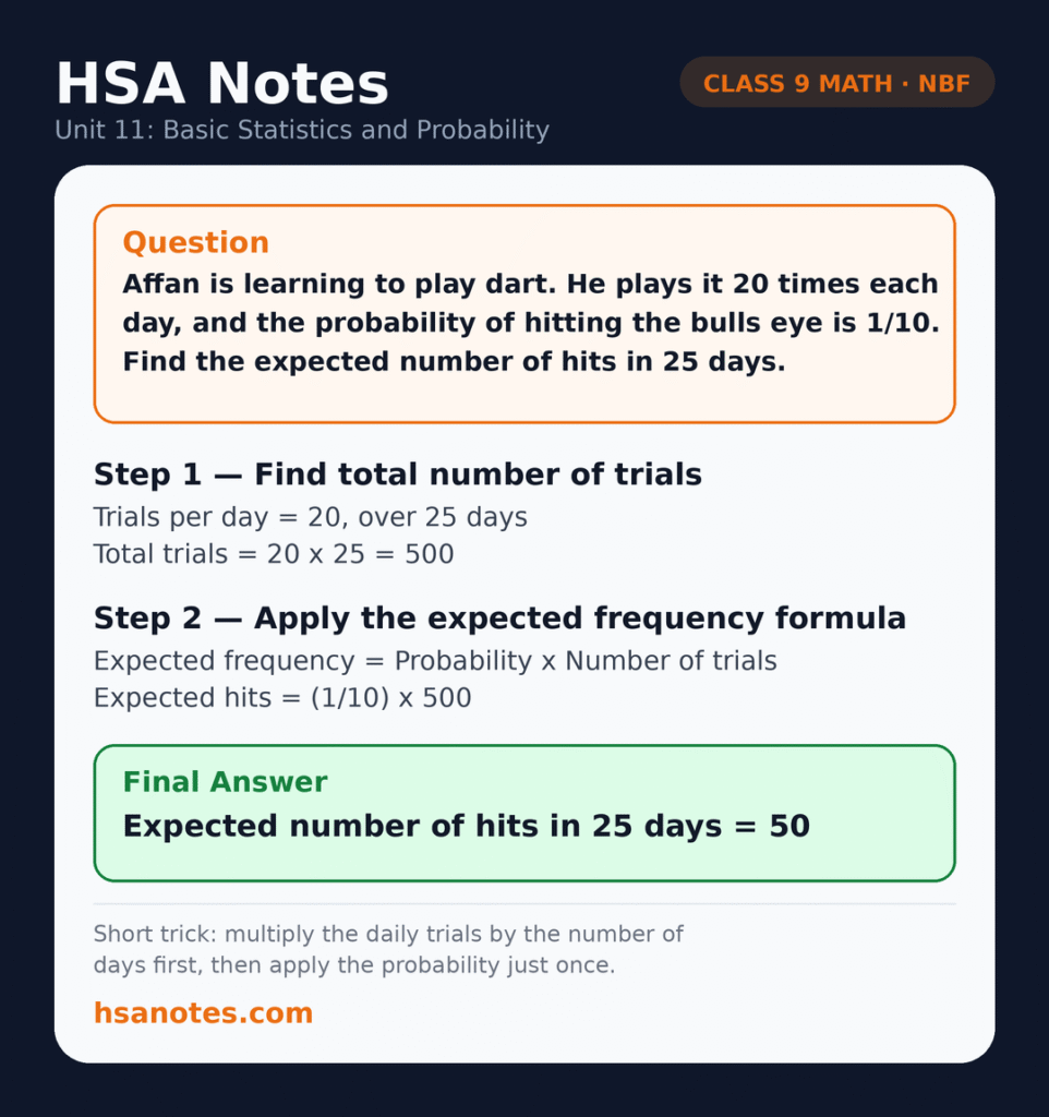
Relative frequency, used as an estimate of probability from experimental data, is Relative Frequency = (frequency of an event occurring) ÷ (total number of trials). Expected frequency predicts how often an event should occur over a number of trials, based on its probability: Expected Frequency = Probability × Number of trials.
Worked Examples
Example 1 (Mean for grouped/repeated data): Find the mean of x = 2, 3, 1, 2, 2, 3, 2, 3, 4, 2, 5, 2, 3, 4, 5, 2, 1, 3, 5, 1 using frequencies.
Frequencies: 1 occurs 3 times, 2 occurs 7 times, 3 occurs 5 times, 4 occurs 2 times, 5 occurs 3 times.
Σfx = (1×3) + (2×7) + (3×5) + (4×2) + (5×3) = 3 + 14 + 15 + 8 + 15 = 55. n = 3+7+5+2+3 = 20.
Mean = 55 ÷ 20 = 2.75.
Example 2 (Median, ungrouped): Find the median of 1075, 1050, 2050, 1030, 2045, 1090, 1530.
Arranged in order: 1030, 1050, 1075, 1090, 1530, 2045, 2050. With n = 7 (odd), median is the 4th value = Rs. 1090.
Example 3 (Mode): Find the mode of 30, 25, 40, 30, 45, 25, 30, 40, 30.
30 occurs most often (4 times), so the mode is 30 (unimodal data).
Example 4 (Single event probability): A cubical die is rolled once. Find the probability of getting a number greater than 4.
Sample space = {1,2,3,4,5,6}, favourable outcomes = {5,6}, so P = 2/6 = 1/3.
Example 5 (Relative frequency): A fair coin is tossed 150 times and heads come up 70 times. Find the relative frequency of getting heads.
Relative Frequency = 70 ÷ 150 = 7/15 ≈ 0.467.
Important Formulas at a Glance
| Concept | Formula |
|---|---|
| Mean (ungrouped) | x̄ = Σx ÷ n |
| Mean (grouped/frequency) | x̄ = Σfx ÷ Σf |
| Median (odd n) | ((n+1)/2)th value |
| Median (grouped) | l + (h/f)(n/2 − c) |
| Complementary probability | P(E’) = 1 − P(E) |
| Relative frequency | f ÷ n (favourable ÷ total trials) |
| Expected frequency | Probability × Number of trials |
Exercises in Unit 11
| Exercise | Main Focus |
|---|---|
| 11.1 | Frequency distribution tables, histograms, frequency polygons |
| 11.2 | Mean, median, and mode for ungrouped and grouped data |
| 11.3 | Single event and complementary event probability, relative and expected frequency |
| Review Exercise 11 | MCQs, short and long questions |
Exam Tips
- Always arrange the data in order before finding the median.
- Remember that mode can have more than one value (or none), unlike mean and median.
- Use class boundaries, not class limits, when drawing a histogram with continuous data.
- For grouped data formulas (mean, median, mode), identify l, h, f, n, and c carefully before substituting.
- Check that P(E) + P(E’) always equals 1 as a quick way to verify your probability answer.
About HSA Notes
HSA Notes is a free educational platform for secondary and higher secondary students in Pakistan. It publishes solved notes, model papers, and study material aligned with the NBF, PECTAA, PCTAA, and FBISE curricula, covering Mathematics, Physics, Chemistry, Biology, Computer Science, and English. Our solutions are written by our own team, giving students clear, original, step-by-step help.
Online Classes
Students who want guided learning can join our online classes run by Hamdard Science Academy. The classes follow the new NBF book unit by unit, so Unit 11 concepts, examples, and exercises are taught in a clear order alongside these notes. To ask about the schedule, fees, or admission, email hsanotes48@gmail.com.
Conclusion
Basic Statistics and Probability brings together data representation, averages, and the basics of chance in one large, practical unit. With steady practice distinguishing mean, median, and mode, and clear understanding of probability rules, this unit becomes very manageable despite its size. Free solved exercises and PDF notes are available on HSA Notes, and online classes are there if you need extra support.